The No-Time Universe (NTU) Framework

Fractal Coarse-Graining and the emergence of physical Reality

Working Theoretical Framework — Version 2026

---

1. Abstract

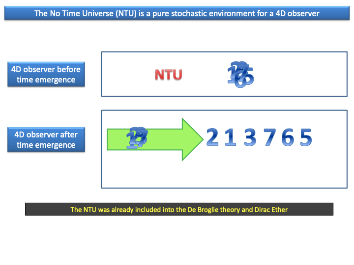
The No-Time Universe (NTU) framework proposes that spacetime, causality and observable physical laws are not fundamental components of reality, but emergent structures arising from a deeper atemporal relational substrate.

Within this approach:

• Quantum Mechanics and General Relativity describe different organizational levels of reality,
• time is not fundamental,
• Lorentzian spacetime is emergent,
• and physical observables arise through large-scale statistical organization and fractal coarse-graining.

The NTU substrate is assumed to be:

• discrete,
• relational,
• isotropic,
• non-local,
• Euclidean,
• and fundamentally without temporal ordering.

Observable physics appears only after recursive averaging processes acting across scales.

The framework introduces:

• pre-link relational structures,
• fractal connectivity surfaces,
• emergent causality,
• statistical reconstruction of time,
• and relativistic geometry as a stable coarse-grained phase.

The central mechanism of NTU is fractal coarse-graining, through which:

• quantum mechanics,
• relativity,
• gravity,
• probability,
• and temporal flow emerge simultaneously from a deeper non-temporal substrate.

---

2. Foundational Principle

Two levels of reality

The central axiom of NTU is: Quantum Mechanics and General Relativity may describe two distinct levels of reality rather than two incompatible descriptions of the same physical object.

Within this interpretation:

Object 1 : observable Physics	Object 2 : NTU Substrate
Lorentzian spacetime	Pre-geometric relational structure based on a fundamentally Euclidean and rigid geometry, reminiscent of the pre-relativistic geometric concepts discussed by Einstein in his presentation of relativity :” Euclidean geometry describes pure rigid objects”.
Causal events	Possible relational configurations existing prior to the emergence of determined causality. The absence of fully determined causal ordering naturally leads to stochastic and probabilistic behavior at the observable level. The NTU shows all the characteristics of Dirac Ether.
Observable time	Atemporal organization
Continuous geometry	Discrete fractal structure
Classical locality	Non-local connectivity
Energy transfer fixing causality	Pre-links before transfer : a new vision of de Broglie pilote wave fixing challenges of original dB waves.

Observable reality emerges at the interface between these two domains.

---

3. The NTU substrate

The NTU substrate is modeled as a discrete relational structure:

$NTU=(V,E,C,R)$

Where:

• $V$ represents elementary nodes,
• $E$ possible relations,
• $C$ the configuration space,
• $R$ recursive transition rules.

At this level:

• no fundamental time exists,
• no global causal ordering exists,
• no Lorentzian geometry exists,
• and no preferred frame exists.

The substrate is fundamentally isotropic and reciprocal. The elementary physical object is not a particle or a field, but a surface of pre-links:

$\Sigma_n \subset V$

These pre-link structures represent possible relational organizations before realized energy transfer.

4. Quantization of Newton formula

The NTU framework assumes that two fundamental quantizations of Newtonian mechanics naturally emerge at the discrete substrate level.

The first quantization corresponds to the elastic collision relation reformulated through discrete Planck-scale momentum units. Within the NTU framework, momentum is expressed as:

$m v = N m_P c$

Where:

• $m$ is the observable mass,
• $v$ the effective velocity,
• $m_P$​ the Planck mass,
• $c$ the speed of light,
• and $N$ a dimensionless discrete scaling parameter.

The parameter $N$ is defined by:

$N = 2\pi \times n_{dB} \times \ell_P$

Where:

• $n_{dB}$​ represents the number of de Broglie wavelengths involved in the relational structure,
• $\ell_P$​ is the Planck length.

Within NTU, this relation suggests that observable momentum emerges from discrete Planck-scale relational units organized through fractal connectivity through multiple elastic collisions with a rigid structure.

Momentum is therefore no longer interpreted as a purely continuous quantity, but as the macroscopic manifestation of an underlying discrete relational organization.

---

The second quantization concerns gravitation itself, which is no longer interpreted as a continuous force field acting through spacetime, but as a statistical organization of relational links between discrete configurations.

The classical Newtonian interaction:

$F=G\frac{m_1 m_2}{r^2}$

is reformulated in NTU as a connectivity relation between pre-link structures:

$L_G(i,j)\propto\frac{m_i m_j}{d_{ij}^2}$

Where:

• $L_G(i,j)$ represents the density of gravitational relational links,
• $d_{ij}$is an effective relational distance inside the substrate.

Within this perspective, gravitational interaction becomes a large-scale manifestation of microscopic connectivity density inside the NTU substrate.

---

A fundamental dimensionless couple of parameters based on N and 1/N are then introduced:

$$N_Q=\frac{\ell_P}{\lambda_{dB}}$$$$N_G=\frac{\lambda_{dB}}{\ell_P}$$

where:

• $\lambda_{dB}$is the de Broglie wavelength,
• $\ell_P$ is the Planck length.

This ratio defines the transition between discrete microscopic organization and effective continuous physics.

---

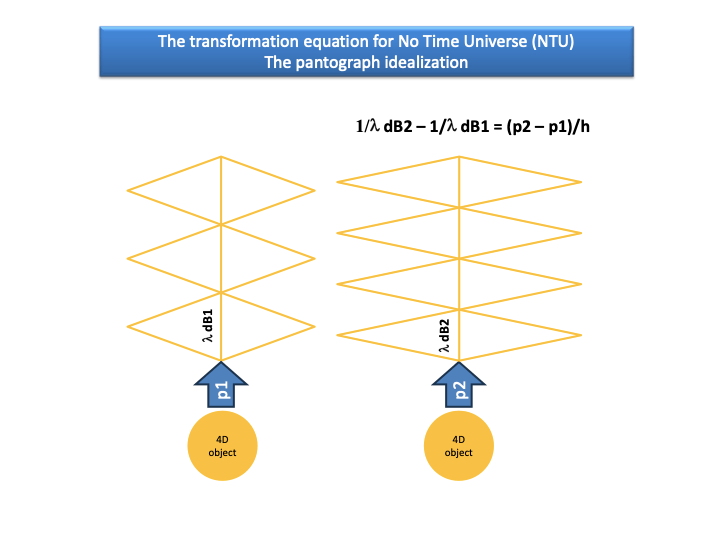
The NTU framework further introduces the pantograph principle, a recursive scaling mechanism based on two coupled relational axes. At the substrate level, these axes do not yet represent physical spacetime coordinates, but rather scale propagation and relational organization inside the pre-geometric structure.

The associated transformation law is therefore neither a Galilean transformation nor a Lorentz transformation. Instead, NTU proposes a specific relational scaling transformation emerging from the recursive organization of the substrate itself. This transformation law is closely related to the scaling behavior already observed in the transformation properties of de Broglie waves.

While Galilean transformations preserve absolute time and Lorentz transformations preserve relativistic spacetime intervals, the NTU transformation acts on relational scale structures prior to the emergence of spacetime geometry. Observable relativistic transformations are interpreted as effective large-scale limits of this deeper pantograph dynamics after symmetry breaking and fractal coarse-graining.

The general transformation may be formally represented as:

$\mathcal{P}_N:(x_1,x_2)\rightarrow(Nx_1,\frac{1}{N}x_2)$

Following symmetry breaking, these dual recursive axes progressively generate effective temporal coordinates and relativistic spacetime organization.

At the fundamental substrate level, these axes do not yet represent physical time. They instead describe scale propagation and relational organization inside the pre-geometric structure.

Following symmetry breaking and large-scale coarse-graining, these two recursive axes progressively generate:

• temporal ordering,
• causal asymmetry,
• and effective relativistic time coordinates.

Observable spacetime is therefore interpreted as the macroscopic projection of a deeper dual-scale relational structure. In the NTU framework, the de Broglie phase harmony relation is interpreted as the observable projection of the pantographic transformation of the NTU substrate.
The quantum axis and the gravitational axis transform inversely through the Lorentz factor, producing the simultaneous appearance of γ and 1/γ in relativistic wave-particle relations.
The wave frequency corresponds to the quantum branch of the pantograph, while inertial mass corresponds to the gravitational branch.

---

5. Why the NTU structure must be fractal

NTU assumes that the substrate cannot be smooth or differentiable at the fundamental scale. If not, microscopic reality were already continuous:

• quantum indeterminacy would disappear,
• scale transitions would become trivial,
• and emergent spacetime would already be implicitly assumed.

Instead, NTU proposes:

• recursive self-similarity,
• scale dependence,
• and non-differentiable connectivity.

The substrate therefore behaves as a fractal relational geometry.

This fractality is essential because:

• quantum behavior naturally emerges from non-differentiable relational paths,
• while classical behavior corresponds to smooth effective trajectories generated through large-scale averaging.

---

6. Recursive Dynamics of Pre-Link Structures

Microscopic evolution is described recursively:

$\Sigma_{n+1}=\Sigma_n \cup \bigcup_{i=1}^{M}\lambda_i(u)R_i(\Sigma_n)\cup \eta_n$

Where:

• $R_i$Ri​ are reconnection or symmetry operators,
• $\lambda_i(u)$λi​(u) are scale-dependent contraction or expansion factors,
• $\eta_n$ηn​ represents stochastic fluctuations.

This recursive process generates:

• self-similar connectivity,
• fractal organization,
• and fluctuating relational geometries.

At this stage:

• time does not yet exist,
• causality does not yet exist,
• and trajectories are not fundamental entities.

Only relational organization exists.

---

7. Fractal Coarse-Graining

7.1 The principle of NTU central mechanism

Fractal coarse-graining is the core mechanism of the NTU framework. In conventional physics, coarse-graining smooths microscopic fluctuations in order to recover effective macroscopic laws. In the NTU framework, this is the bridge between:

• the atemporal microscopic substrate of pre-links,
• and the observable macroscopic Universe governed by spacetime, causality, quantum mechanics and gravity.

In NTU, neither time nor spacetime are fundamental entities. What fundamentally exists is a discrete relational substrate composed of fluctuating configurations of connectivity. Observable physics only emerges after a multi-scale averaging process — the coarse-graining of this substrate.

NTU extends this concept radically. The process does not average particles evolving in spacetime. Instead, it averages:

• pre-geometric relational configurations,
• fractal connectivity structures,
• and possible energy-transfer pathways.

The coarse-graining scale satisfies:

$\ell_P \ll \ell \ll L_{obs}$

Where:

• $\ell_P$ is the Planck scale,
• $L_{obs}$​ the macroscopic observational scale.

Observable physics appears only after recursive averaging across these scales.

7.2 NTU Coarse-Graining final version : Unified Quantum and Gravitational evolution functions

7.2.1 Pantographic fractal geometry

The NTU geometry is built upon two reciprocal pantographic axes: a quantum axis and a gravitational axis.

The gravitational pantographic factor is defined as$$N_G = \frac{\ell_P}{\lambda_{dB}},$$

where $\ell_P$ denotes the Planck length and $\lambda_{dB}$​ the local de Broglie wavelength.

The quantum pantographic factor is defined as the reciprocal quantity$$N_Q = \frac{\lambda_{dB}}{\ell_P}.$$

The two factors satisfy the fundamental pantographic constraint$$N_G N_Q = 1.$$

The factor $N_G$has a direct physical interpretation. It represents the number of hidden NTU iterations—or equivalently the number of quantum bursts in the sense of Queirós-Conde—required to generate a single observable Planck-scale event.

Accordingly,$$N_G=n.$$

In the gravitational regime, the de Broglie wavelength becomes smaller than the Planck length:$$\lambda_{dB} < \ell_P.$$

Consequently,$$N_G = \frac{\ell_P}{\lambda_{dB}} > 1,$$

which means that several hidden NTU iterations must accumulate before an observer living in the four-dimensional universe can detect an elementary displacement of one Planck length.

The Planck threshold is reached when$$N_G \lambda_{dB} = \ell_P.$$

The factor $N_Q$NQ​ is the reciprocal pantographic scale:$$N_Q = \frac{1}{N_G}.$$

It describes the complementary projection associated with the quantum axis.

While $N_G$counts the hidden closure iterations responsible for the emergence of measurable events, $N_Q$characterizes the reciprocal geometric projection generated by the pantographic structure.

The pantographic transformation can therefore be written as$$\mathcal{P} : (\tau_Q,\tau_G) \longrightarrow (N_Q\,\tau_Q,\; N_G\,\tau_G),$$

with$$N_GN_Q=1.$$

This reciprocal mapping expresses the central duality of the NTU framework:$$\text{Quantum projection} \quad\Longleftrightarrow\quad \text{Gravitational accumulation},$$

and conversely,$$\text{Quantum accumulation} \quad\Longleftrightarrow\quad \text{Gravitational projection}.$$

The interpretation becomes particularly clear in the context of quantum bursts.

Following Queirós-Conde, the observable duration is reconstructed from a sequence of elementary de Broglie pulsations:$$\tau = n\,\tau_{dB}.$$

Within the NTU framework, this relation becomes$$\tau = N_G\,\tau_{dB},$$

showing that the gravitational pantographic factor $N_G$NG​ is precisely the number of hidden bursts required to reconstruct an observable event.

This identification establishes a direct bridge between the NTU pantographic geometry and the quantum burst formalism of Fractal Thermodynamics.

---

Both pantographics axes functions :$$F_Q = N_Q^{1/2}\Sigma_Q$$$$F_G = N_G^{1/2}\Sigma_G$$

This transformation constitutes the fundamental dynamical law of the NTU.

The associated fractal coefficient is:$$N_k = \sqrt{\frac{1}{N}}$$

The resulting fractal surface generated by the substrate is:$$\Sigma(N) = \ell_P^2 N^{D_{\mathrm{eff}}}$$

with:$$D_{\mathrm{eff}} \simeq 2.1$$

---

7.2.2 Open and Closed fractal surfaces

The total fractal surface is divided into two complementary sectors.

The open pilot surface is:$$\Sigma_Q = \chi \Sigma(N)$$

The closed rigidified surface is:$$\Sigma_G = (1-\chi) \Sigma(N)$$

where:$$\chi = \frac{\Sigma_{\mathrm{open}}} {\Sigma_{\mathrm{open}} + \Sigma_{\mathrm{closed}}}$$

is the non-closure coefficient.

Its complement:$$1-\chi$$

represents the closure ratio.

---

7.2.3 The fundamental NTU equation

The fundamental NTU variable is a generated volume:$$V_{\mathrm{NTU}}.$$

The reason is that the two evolution functions $F_Q$​ and $F_G$ are effective fractal surfaces generated on the two pantographic axes crossed by the causal front.

In the gravitational regime, the de Broglie wavelength becomes smaller than the Planck length. To meet the Planck length, the gravitational accumulation factor is:$$N_G = \frac{\ell_P}{\lambda_{dB}},$$

while the quantum reciprocal factor is:$$N_Q = \frac{\lambda_{dB}}{\ell_P}.$$

They satisfy$$N_G N_Q = 1.$$

In the gravitational regime,$$\lambda_{dB}<\ell_P,$$

therefore$$N_G>1.$$

The factor $N_G$ represents the number of hidden NTU bursts (accumulation factor) required to generate one observable Planck-scale event:$$N_G=n.$$

The quantum and gravitational fractal surfaces are defined as$$\Sigma_Q = \chi\,\ell_P^2 N_Q^{D_{\mathrm{eff}}},$$

and$$\Sigma_G = (1-\chi)\,\ell_P^2 N_G^{D_{\mathrm{eff}}}.$$

The corresponding evolution surfaces are$$F_Q = N_Q^{1/2}\Sigma_Q,$$

which gives$$F_Q = \chi\,\ell_P^2 N_Q^{D_{\mathrm{eff}}+\frac12},$$

and$$F_G = N_G^{1/2}\Sigma_G,$$

which gives$$F_G = (1-\chi)\,\ell_P^2 N_G^{D_{\mathrm{eff}}+\frac12}.$$

The effective NTU surface swept by the causal front is therefore$$\Sigma_{\mathrm{eff}}^{\mathrm{NTU}} = F_Q+F_G.$$

The elementary NTU displacement is the local de Broglie wavelength:$$\Delta_{\mathrm{NTU}} = \lambda_{dB}.$$

Thus, the fundamental NTU volume-generation equation is$$\Delta V_{\mathrm{NTU}} = \Sigma_{\mathrm{eff}}^{\mathrm{NTU}} \Delta_{\mathrm{NTU}}.$$

Equivalently,$$\Delta V_{\mathrm{NTU}} = (F_Q+F_G)\lambda_{dB}.$$

Substituting the explicit forms gives$$\Delta V_{\mathrm{NTU}} = \ell_P^2 \left[ \chi N_Q^{D_{\mathrm{eff}}+\frac12} + (1-\chi) N_G^{D_{\mathrm{eff}}+\frac12} \right] \lambda_{dB}.$$

For a four-dimensional observer, the hidden NTU bursts are not individually observable. The observable Planck threshold is reached when$$N_G\lambda_{dB} = \ell_P.$$

Therefore, one observable 4D volume increment corresponds to$$\Delta V_{4D} = N_G \Delta V_{\mathrm{NTU}}.$$

Using$$N_G\lambda_{dB} = \ell_P,$$

one obtains$$\Delta V_{4D} = (F_Q+F_G)\ell_P.$$

Thus,$$\Delta V_{4D} = \ell_P^3 \left[ \chi N_Q^{D_{\mathrm{eff}}+\frac12} + (1-\chi) N_G^{D_{\mathrm{eff}}+\frac12} \right].$$

This is the Planck-scale projection perceived by an observer living in the four-dimensional universe.

---

7.2.4 Coarse-Graining

The discrete NTU dynamics is therefore written as$$V_{n+1}^{\mathrm{NTU}} – V_n^{\mathrm{NTU}} = (F_Q+F_G)\lambda_{dB}.$$

For a 4D observer, this becomes$$V_{n+1}^{4D} – V_n^{4D} = (F_Q+F_G)\ell_P.$$

The continuous limit is obtained by averaging many hidden NTU bursts:$$N_G \rightarrow \infty,$$$$\lambda_{dB} \rightarrow 0,$$

with the observable Planck threshold preserved:$$N_G\lambda_{dB} = \ell_P.$$

The coarse-grained volume dynamics becomes$$dV_{4D} = (F_Q+F_G)\,d\ell,$$

where$$d\ell = c\,dt.$$Therefore,$$dV_{4D} = c(F_Q+F_G)\,dt.$$

Substituting the explicit expressions gives$$dV_{4D} = c\ell_P^2 \left[ \chi N_Q^{D_{\mathrm{eff}}+\frac12} + (1-\chi) N_G^{D_{\mathrm{eff}}+\frac12} \right]dt.$$

The stochastic term arises because a four-dimensional observer cannot distinguish all intermediate open pre-link configurations. The unresolved fraction is measured by$$\chi = \frac{\Sigma_{\mathrm{open}}} {\Sigma_{\mathrm{open}}+\Sigma_{\mathrm{closed}}}.$$

Thus the coarse-grained stochastic equation is$$dV_{4D} = c(F_Q+F_G)\,dt + \chi\,G_0(V)\,dW_t.$$

The corresponding Fokker–Planck equation for the probability density $P(V,t)$P(V,t) is$$\frac{\partial P}{\partial t} = – \frac{\partial}{\partial V} \left[ c(F_Q+F_G)P \right] + \frac12 \frac{\partial^2}{\partial V^2} \left[ \chi^2G_0^2(V)P \right].$$

The diffusion coefficient is therefore$$D(V) = \frac12 \chi^2G_0^2(V).$$

Conclusion

This shows that the Brownian component is not introduced arbitrarily. It emerges from the projection of unresolved open NTU configurations into a four-dimensional continuous description. The conceptual chain is therefore$$\text{fractal surfaces} \rightarrow \text{hidden NTU bursts} \rightarrow \text{causal-front sweeping} \rightarrow \text{volume generation} \rightarrow \text{4D coarse-graining} \rightarrow \text{Fokker–Planck dynamics}.$$

The NTU does describe the generation of a volume $V_{\mathrm{NTU}}$by the causal front sweeping fractal pre-link surfaces.

7.3 First version of Coarse-Graining derivation of the NTU dynamics (history of NTU)

The objective of the coarse-graining procedure is to move from the microscopic NTU dynamics — defined as a sequence of discrete impacts between 4D objects and Planck-scale NTU nodes — toward an effective continuous description compatible with standard quantum and relativistic physics.

The NTU substrate is assumed to be composed of rigid Planck-scale nodes. A 4D object interacting with this substrate generates, at each microscopic collision, two coupled effects:$$\boxed{ \text{pre-link generation on the quantum axis} }$$

and$$\boxed{ \text{energy/momentum transfer on the gravitic axis} }$$​

The fundamental state of the NTU substrate at iteration n is represented by:

X(n) = ( p(n) , Σ(n) )

where:

• p(n) represents the quantum branch of the pantograph and describes the fractal surface of possible configurations.
• Σ(n) represents the gravitational branch and describes the rigidified surface generated by closed pre-links.

The non-closure coefficient is:$$\chi_n = \frac{\Sigma_{\mathrm{open},n}} {\Sigma_{\mathrm{open},n} + \Sigma_{\mathrm{closed},n}}$$

The closure coefficient is:$$1-\chi_n = \frac{\Sigma_{\mathrm{closed},n}} {\Sigma_{\mathrm{open},n} + \Sigma_{\mathrm{closed},n}}$$

The pantographic scaling parameter is:$$N = \frac{\lambda_{dB}} {\ell_P}$$

The associated fractal coefficient is:$$N_k = \sqrt{\frac{1}{N}}$$Nk​=N1​​

The quantum function is defined as:$$F_Q(X_n,N) = N\,N_k\, \mathcal{F}_Q(p_n)$$

Substituting $N_k$Nk​ gives:$$F_Q(X_n,N) = \sqrt{N}\, \mathcal{F}_Q(p_n)$$

The gravitational function is defined as:$$F_G(X_n,N) = \frac{1}{N}\, N_k\, \mathcal{F}_G(\Sigma_n)$$

Substituting $N_k$Nk​ gives:$$F_G(X_n,N) = \frac{1}{N^{3/2}}\, \mathcal{F}_G(\Sigma_n)$$

The fundamental NTU evolution equation then becomes:$$X_{n+1} – X_n = \Big[ \chi_n F_Q(X_n,N) + (1-\chi_n) F_G(X_n,N) \Big] \Delta_{\mathrm{NTU}}$$

Substituting the two pantographic functions yields:$$X_{n+1} – X_n = \Bigg[ \chi_n \sqrt{N}\, \mathcal{F}_Q(p_n) + (1-\chi_n) \frac{1}{N^{3/2}} \mathcal{F}_G(\Sigma_n) \Bigg] \Delta_{\mathrm{NTU}}$$

This formulation possesses three important properties.

First, the pantograph appears explicitly through the reciprocal scaling factors:$$N$$

and$$\frac{1}{N}$$

which define the dual evolution of the quantum and gravitational branches.

Second, the fractal coefficient:$$N_k = \sqrt{\frac{1}{N}}$$

remains explicitly embedded in both branches of the dynamics.

Third, the non-closure coefficient:$$\chi_n$$

weights exclusively the quantum pilot surface associated with open pre-links, while:$$1-\chi_n$$

weights exclusively the gravitational rigidified surface associated with closed pre-links.

Consequently, the evolution of the substrate is entirely governed by the balance between open and closed configurations. The quantum branch dominates when the fraction of open pre-links is large, whereas the gravitational branch progressively dominates as closure and rigidification increase.

This equation therefore provides a compact mathematical expression of the NTU coarse-graining process before projection toward the effective 4D description and the subsequent emergence of Langevin and Fokker–Planck dynamics.

7.4 NTU observer versus 4D observer : move from NTU coarse graining (discret) to Fokker Planck (initial version)

For an observer located at the NTU substrate level, both open and closed surfaces are directly accessible. The NTU observer can observe:

• Σopen
• Σclosed

and therefore has access to the complete geometrical state of the system. No stochastic interpretation is required. The apparent uncertainty simply corresponds to the coexistence of multiple unresolved configurations.

For an observer living in the emergent 4D spacetime, only the rigidified sector:

Σclosed

is directly observable.

The unresolved configurations:

Σopen

exist at scales below the effective observational resolution associated with the Planck length and therefore remain inaccessible. After coarse-graining, their cumulative effect is perceived as an effective Brownian noise.

The emergence chain may therefore be summarized as:

Open surfaces → Hidden configurations → Effective Brownian noise

In the NTU framework, stochasticity is not fundamental. It is the macroscopic projection of unresolved geometrical configurations associated with non-closed pre-links.

For such a NTU observer, the coefficient:$$\chi_n = \frac{\Sigma_{\mathrm{open},n}} {\Sigma_{\mathrm{open},n} + \Sigma_{\mathrm{closed},n}}$$

is not a probability and not a noise term. It is a direct geometrical ratio measuring the fraction of non-closed pre-links. However, a 4D observer does not have access to:$$\Sigma_{\mathrm{open},n}$$

The 4D observer only observes the rigidified sector:$$\Sigma_{\mathrm{closed},n}$$

The non-closed configurations remain hidden because their effective displacements or fractal thicknesses lie below the observational resolution associated with the Planck scale:$$\delta_{\mathrm{NTU}} < \ell_P$$

or, equivalently, below the associated Planck time resolution:$$\Delta t_{\mathrm{NTU}} < t_P$$

As a consequence, the 4D observer cannot distinguish the individual transitions between different open fractal configurations. The unresolved open surface is therefore replaced by an effective stochastic process. The NTU displacement:$$\Delta_{\mathrm{NTU}}$$

is projected as a 4D temporal increment:$$\Delta_{\mathrm{NTU}} \longrightarrow dt$$

and the unresolved variation of the open surface becomes an effective Brownian increment:$$\Sigma_{\mathrm{open}} \longrightarrow dW_t$$

This does not mean that Brownian noise is fundamental. It means that Brownian noise is the 4D statistical projection of unresolved non-closed fractal configurations defining the effective drift.

Now, we introduce 2 new functions compatible with generic stochastic functions. When deriving Langevin and Fokker–Planck equations, the standard mathematical literature usually introduces two generic functions:$$A(X)$$

and$$B(X)$$

leading to the well-known stochastic equation:$$dX = A(X)\,dt + B(X)\,dW_t$$

where:

• $A(X)$ is called the drift term,
• $B(X)$ is called the diffusion term,
• $dW_t$​ is a Brownian increment.

This notation is extremely useful in probability theory because it is completely general:$$A(X) = \chi(X,N) \sqrt{N}\, \mathcal{F}_Q(p) + (1-\chi(X,N)) \frac{1}{N^{3/2}} \mathcal{F}_G(\Sigma)$$

and define the effective diffusion amplitude:$$B(X) = \chi(X,N)\, G_0(X,N)$$

where $G_0(X,N)$measures how strongly unresolved open configurations affect the 4D observable state.

The projected 4D dynamics is then written as a Langevin equation:$$dX = A(X)\,dt + B(X)\,dW_t$$

where:$$dW_t$$

is an effective Brownian increment generated by the coarse-graining of inaccessible open fractal surfaces. The associated probability density for a 4D observer is:$$P(X,t)$$

This density does not describe fundamental uncertainty in the NTU substrate. It describes the uncertainty of a 4D observer who cannot resolve the open pre-link configurations.

The Langevin equation:$$dX = A(X)\,dt + B(X)\,dW_t$$

induces the Fokker–Planck equation:$$\frac{\partial P(X,t)} {\partial t} = – \frac{\partial} {\partial X} \left[ A(X)\,P(X,t) \right] + \frac{1}{2} \frac{\partial^2} {\partial X^2} \left[ B^2(X)\,P(X,t) \right]$$

Substituting the NTU diffusion amplitude:$$B(X) = \chi(X,N)\, G_0(X,N)$$

gives:$$\frac{\partial P(X,t)} {\partial t} = – \frac{\partial} {\partial X} \left[ A(X)\,P(X,t) \right] + \frac{1}{2} \frac{\partial^2} {\partial X^2} \left[ \chi^2(X,N)\, G_0^2(X,N)\, P(X,t) \right]$$

The effective diffusion coefficient is therefore:$$D(X) = \frac{1}{2} \chi^2(X,N) G_0^2(X,N)$$

This is the key result. The diffusion coefficient is not fundamental. It is determined by the fraction of non-closed pre-links:$$D(X) \propto \chi^2(X,N)$$

Thus, when the open surface dominates:$$\chi \rightarrow 1$$

the 4D observer sees strong stochastic behavior.

When the closed surface dominates:$$\chi \rightarrow 0$$

the diffusion coefficient vanishes:$$D(X) \rightarrow 0$$D(X)→0

and the effective 4D dynamics becomes deterministic:$$dX = A(X)\,dt$$

The emergence chain is therefore:$$\Sigma_{\mathrm{open}} \longrightarrow \chi \longrightarrow B(X) \longrightarrow D(X) \longrightarrow \mathrm{Fokker\text{-}Planck\ Dynamics}$$

This establishes the NTU interpretation of Brownian noise.

---

Projection Toward a 4D Observer

A 4D observer cannot resolve the individual open configurations contained in:$$\Sigma_{\mathrm{open}}$$

because their characteristic variations occur below the Planck scale:$$\delta_{\mathrm{NTU}} < \ell_P$$δNTU​<ℓP​

or equivalently:$$\Delta t_{\mathrm{NTU}} < t_P$$

As a consequence, the unresolved open configurations become statistically indistinguishable.

The NTU displacement:$$\Delta_{\mathrm{NTU}}$$

is perceived as a temporal increment:$$dt$$

while the unresolved open surface appears as an effective Brownian fluctuation.

The projected 4D equation becomes:$$dX = \Big[ \chi(X,N) F_Q(X,N) + (1-\chi(X,N)) F_G(X,N) \Big]dt + \chi(X,N) G_0(X,N) dW_t$$

where:$$dW_t$$

is an effective Brownian increment. Importantly, this Brownian term is not fundamental. It emerges solely because the observer cannot access the complete set of open fractal configurations.

---

Emergence of the Fokker–Planck equation (first version)

The probability density:$$P(X,t)$$

describes the probability for a 4D observer to measure the state:$$X$$

The corresponding Fokker–Planck equation is obtained directly from the NTU projection:$$\frac{\partial P(X,t)} {\partial t} = – \frac{\partial} {\partial X} \left\{ \left[ \chi(X,N) F_Q(X,N) + (1-\chi(X,N)) F_G(X,N) \right] P(X,t) \right\}$$$$+ \frac{1}{2} \frac{\partial^2} {\partial X^2} \left[ \chi^2(X,N) G_0^2(X,N) P(X,t) \right]$$

No auxiliary functions $A(X)$ or $B(X)$ are required. The physical interpretation remains fully visible throughout the derivation. The quantum branch, the gravitational branch, and the non-closure coefficient all remain explicitly present.

---

Physical Interpretation

The complete emergence chain is therefore:$$\Sigma_{\mathrm{open}} \longrightarrow \chi \longrightarrow \chi\,G_0 \longrightarrow \mathrm{Brownian\ Projection} \longrightarrow \mathrm{Fokker\text{-}Planck\ Dynamics}$$

The Brownian process is not a fundamental ingredient of reality.

It is the effective 4D manifestation of unresolved open configurations.

Likewise, the Fokker–Planck equation is not fundamental.

It is the statistical description seen by a 4D observer after projecting the deeper NTU pantographic dynamics onto emergent spacetime.

In this interpretation:$$\text{Fractal Thermodynamics}$$

describes the geometry of the open pilot surface,

while$$\text{Stochastic Gravity}$$

describes the fluctuations associated with the rigidified surface.

Both originate from the same underlying process of pre-link closure governed by the NTU fractal pantograph.

The coarse-graining limit now has two natural asymptotic regimes.

In the quantum regime:$$N\ll1$$

the diffusion term dominates:$$\frac{1}{N^{2\beta}} \gg1$$

and the system is governed by broad pre-link fluctuations. This corresponds to a non-classical, probabilistic propagation regime.

In the gravitic regime:$$N\gg1$$

the diffusion term becomes suppressed:$$\frac{1}{N^{2\beta}} \rightarrow0$$

and the Fokker–Planck equation reduces to:$$\frac{\partial P}{\partial t} = – \nabla_X\cdot \left[ F_a(X;N)P \right]$$

which is the deterministic transport equation.

This is the emergence of classical motion from the NTU micro-dynamics.

The Schrödinger regime appears when the stochastic pre-link contribution is rewritten through a complex amplitude:$$P(X,t)=|\Psi(X,t)|^2$$

and when the diffusion coefficient is identified with:$$D_Q = \frac{\hbar}{2m}$$

The stochastic continuity equation becomes:$$\frac{\partial P}{\partial t} + \nabla\cdot(Pv) = 0$$

with:$$v=\frac{\nabla S}{m}$$

Introducing:$$\Psi = \sqrt{P} \exp\left(\frac{iS}{\hbar}\right)$$

one obtains the Madelung form:$$\frac{\partial S}{\partial t} + \frac{(\nabla S)^2}{2m} + V + Q = 0$$

where:$$Q = – \frac{\hbar^2}{2m} \frac{\nabla^2\sqrt{P}}{\sqrt{P}}$$

is the quantum potential.

Combining the continuity equation and the Hamilton–Jacobi equation with the quantum potential gives:$$\boxed{ i\hbar \frac{\partial \Psi}{\partial t} = – \frac{\hbar^2}{2m} \nabla^2\Psi + V\Psi }$$

Thus the Schrödinger equation appears as the linear coarse-grained representation of the underlying discrete NTU dynamics.

The key interpretation is:$$\boxed{ \text{the Schrödinger equation is not fundamental;} }$$

rather:$$\boxed{ \text{it is the linear statistical limit of NTU pre-link dynamics.} }$$

In the gravitic limit, the same coarse-graining procedure suppresses the quantum diffusion term and retains only the deterministic flow of momentum. The effective classical action becomes:$$S = \int L\,dt$$

with:$$L=T-V$$

and the condition:$$\delta S=0$$

The Euler–Lagrange equation follows:$$\boxed{ \frac{d}{dt} \left( \frac{\partial L}{\partial \dot{x}} \right) – \frac{\partial L}{\partial x} = 0 }$$

Using:$$p= \frac{\partial L}{\partial \dot{x}}$$

one recovers Hamiltonian mechanics:$$\dot{x} = \frac{\partial H}{\partial p}$$$$\dot{p} = – \frac{\partial H}{\partial x}$$

Thus the NTU coarse-graining produces two effective limits:$$\boxed{ N\ll1 \Rightarrow \text{quantum probabilistic regime} }$$

and:$$\boxed{ N\gg1 \Rightarrow \text{classical/gravitic deterministic regime} }$$

The closed NTU coarse-graining chain is therefore:

1) discrete NTU impacts

2) pantographic inverse scaling

3) fractal surface propagation

4) stochastic pre-link dynamics

5) Fokker–Planck equation

6) Schrödinger / Hamilton / Einstein limits​

The essential result is that the same microscopic update law produces both quantum and classical behavior depending only on the ratio:$$\frac{\lambda_{dB}}{L_P}$$

or equivalently:$$\frac{p}{m_Pc}$$

This provides a closed mathematical bridge between the discrete NTU substrate and the effective continuous laws observed in the 4D universe.

8. From NTU lagrangien to NTU tensor and action : projections toward quantum pilot-wave dynamics where quantum and gravitation are emergent

8.1 Reminder : fundamental NTU Geometry

The NTU geometry is built upon two reciprocal pantographic axes: a quantum axis and a gravitational axis.

The gravitational pantographic factor is defined as$$N_G = \frac{\ell_P}{\lambda_{dB}},$$

where $\ell_P$ denotes the Planck length and $\lambda_{dB}$​ the local de Broglie wavelength.

The quantum pantographic factor is defined as the reciprocal quantity$$N_Q = \frac{\lambda_{dB}}{\ell_P}.$$

The two factors satisfy the fundamental pantographic constraint$$N_G N_Q = 1.$$

The factor $N_G$has a direct physical interpretation. It represents the number of hidden NTU iterations—or equivalently the number of quantum bursts in the sense of Queirós-Conde—required to generate a single observable Planck-scale event.

Accordingly,$$N_G=n.$$

In the gravitational regime, the de Broglie wavelength becomes smaller than the Planck length:$$\lambda_{dB} < \ell_P.$$

Consequently,$$N_G = \frac{\ell_P}{\lambda_{dB}} > 1,$$

which means that several hidden NTU iterations must accumulate before an observer living in the four-dimensional universe can detect an elementary displacement of one Planck length.

The Planck threshold is reached when$$N_G \lambda_{dB} = \ell_P.$$

The factor $N_Q$NQ​ is the reciprocal pantographic scale:$$N_Q = \frac{1}{N_G}.$$

It describes the complementary projection associated with the quantum axis.

While $N_G$counts the hidden closure iterations responsible for the emergence of measurable events, $N_Q$characterizes the reciprocal geometric projection generated by the pantographic structure.

The pantographic transformation can therefore be written as$$\mathcal{P} : (\tau_Q,\tau_G) \longrightarrow (N_Q\,\tau_Q,\; N_G\,\tau_G),$$

with$$N_GN_Q=1.$$

This reciprocal mapping expresses the central duality of the NTU framework:$$\text{Quantum projection} \quad\Longleftrightarrow\quad \text{Gravitational accumulation},$$

and conversely,$$\text{Quantum accumulation} \quad\Longleftrightarrow\quad \text{Gravitational projection}.$$

The interpretation becomes particularly clear in the context of quantum bursts.

8.2 Open and Closed NTU Surfaces

The total fractal surface is decomposed into 3 sectors.

The open quantum surface is:$$\Sigma_Q = \chi \Sigma(N)$$

The closed gravitational surface is:$$\Sigma_G = (1-\chi) \Sigma(N)$$

The non-closure coefficient is:$$\chi = \frac{\Sigma_{\mathrm{open}}} {\Sigma_{\mathrm{open}} + \Sigma_{\mathrm{closed}}}$$

The closure coefficient is:$$1-\chi = \frac{\Sigma_{\mathrm{closed}}} {\Sigma_{\mathrm{open}} + \Sigma_{\mathrm{closed}}}$$

Therefore:$$\Sigma_Q = \chi \ell_P^2 N^{D_{\mathrm{eff}}}$$

and:$$\Sigma_G = (1-\chi) \ell_P^2 N^{D_{\mathrm{eff}}}$$

Based on previous coefficients, the NTU dynamics is governed by two geometric processes. The first is associated with unresolved configurations and is described by the quantum surface-generation function$$F_Q = N_Q^{1/2}\Sigma_Q, \tag{126}$$

while the second is associated with realized configurations and is described by the gravitational accumulation function$$F_G = N_G^{1/2}\Sigma_G. \tag{127}$$

Now we consider a third regime named the critical regime when$$F_Q=F_G. \tag{130}$$

This equality defines a geometric equilibrium between openness and closure. It corresponds neither to an unresolved quantum configuration nor to an over-rigidified gravitational configuration. Instead, it defines the unique regime for which the projection from the NTU to the observable four-dimensional Universe is achieved with minimal geometric cost.

The corresponding critical hypersurface is therefore$$\mathcal{C}_{NTU} = \left\{ F_Q=F_G \right\}. \tag{131}$$

This hypersurface separates the quantum and gravitational sectors of the theory and represents the shortest realizable path through the pre-link network.

Because any additional rigidification would require extra closure bursts, trajectories with$$F_G>F_Q$$

necessarily correspond to slower projected evolution. Conversely, configurations with$$F_Q>F_G$$

cannot generate stable observables.

The critical hypersurface therefore defines the maximal propagation regime compatible with observability.

A maximum projected velocity naturally emerges:$$v_{\max} = v\!\left(F_Q=F_G\right). \tag{132}$$

This velocity is not introduced as a postulate. It arises from the geometry itself as the propagation rate associated with the shortest realizable sequence of closures.

The crucial consequence is that every four-dimensional observer reconstructs the same critical hypersurface. Since rigidified distances are invariant geometric objects, the projection of $\mathcal{C}_{NTU}$CNTU​ is itself invariant.

The four-dimensional image of the critical hypersurface is$$\Pi_{4D} \!\left( \mathcal{C}_{NTU} \right) = \mathcal{C}_{4D}. \tag{133}$$

This projected structure possesses exactly the properties expected of a light cone: it separates accessible trajectories from inaccessible ones and defines the maximum propagation velocity permitted in the emergent spacetime.

Consequently,$$\mathcal{C}_{4D} \equiv \text{Light-Cone Structure}. \tag{134}$$

At this stage, the NTU predicts the existence of an invariant maximal velocity and an associated conical hypersurface without invoking spacetime symmetries, Lorentz transformations, or the speed of light itself.

The emergence chain is therefore$$\text{Pre-link Closure} \rightarrow \text{Rigidification} \rightarrow \text{Invariant Distances} \rightarrow F_Q=F_G \rightarrow \mathcal{C}_{NTU} \rightarrow v_{\max} \rightarrow \mathcal{C}_{4D}. \tag{135}$$

This result may be viewed as a geometric precursor of Special Relativity. The identification of $v_{\max}$vmax​ with the physical speed of light and the derivation of Lorentz transformations are subsequent steps that can be addressed once the nature of massless excitations within the NTU has been established.

We added a third sector when Planck length = dB wave length -> the critical sector

---

8.3 NTU Five-Sector Lagrangian, Action, Projector, Tensor, and Physical Projections

8.3.1 The five-sector NTU lagrangian

Extension of the NTU Sector Structure

In the earliest formulations of the No Time Universe (NTU), the geometry of pre-links and fractal surfaces naturally led to the emergence of three fundamental sectors:

1. The Gravitational Sector (Fg > Fq), corresponding to rigidified and accumulated closure surfaces. This sector gives rise to mass, inertia, gravitation, and the classical spacetime structure.
2. The Quantum Sector (Fq > Fg), corresponding to incomplete closures and hidden sub-Planckian iterations. In this regime, observable spacetime has not yet fully emerged.
3. The Critical Sector (Fq = Fg), corresponding to the unique geometric hypersurface separating the quantum and gravitational domains. This sector is identified with the electromagnetic field and the propagation of light.

The present version of the NTU extends this classification by introducing two additional sectors:

4. The Antimatter Sector, interpreted as the orientation-reversed counterpart of the same closure geometry. Antimatter is therefore not a separate ontology, but a conjugate projection of the NTU causal structure.
5. The Open Sector (Quantum Vacuum), corresponding to pre-links that remain unclosed. These unrealized geometric possibilities form the NTU quantum vacuum and may contribute to the effective vacuum pressure observed in cosmology.

The No Time Universe framework is based on the idea that observable physics emerges from a timeless geometric substrate made of pre-links, fractal surfaces, and a causal front. The dynamics of this substrate is encoded in a five-sector Lagrangian:$$\mathcal L_{\mathrm{NTU}} = \mathcal L_{\mathrm{opt}} + \mathcal L_{\mathrm{crit}} + \mathcal L_{\mathrm{rigid}} + \mathcal L_{\mathrm{anti}} + \mathcal L_{\mathrm{open}} . \tag{1}$$

The critical NTU field is defined as$$\Phi_{\mathrm{NTU}} = F_Q-F_G . \tag{2}$$

The optimality sector is$$\mathcal L_{\mathrm{opt}} = \alpha\, G_{\mathrm{NTU}}^{AB} \nabla_A\Phi_{\mathrm{NTU}} \nabla_B\Phi_{\mathrm{NTU}} . \tag{3}$$

This term encodes the principle that, among all pre-connected events, the causal front selects the most optimal pre-links for closure. It is the NTU equivalent of a geometric least-action principle before the emergence of time.

The critical sector is$$\mathcal L_{\mathrm{crit}} = \beta \left( F_Q-F_G \right)^2 . \tag{4}$$

Its minimum is reached when$$F_Q=F_G . \tag{5}$$

This condition defines the critical hypersurface of the NTU. This sector gives rise to the electromagnetic field after 4D projection.

The rigidified sector is$$\mathcal L_{\mathrm{rigid}} = \gamma\, \mathbb S_{AB}\mathbb S^{AB}. \tag{6}$$

This term describes closed and rigidified pre-link surfaces. It carries the emergence of mass, inertia, relativistic slowing, and gravitation.

The antisymmetric sector is$$\mathcal L_{\mathrm{anti}} = -\frac14 \mathbb A_{AB}\mathbb A^{AB}. \tag{7}$$

This term describes oriented critical structures. After projection, it becomes the Maxwell Lagrangian.

The open-sector term is$$\mathcal L_{\mathrm{open}} = \eta \left( 1-\rho_{\mathrm{closed}} \right). \tag{8}$$

This term accounts for pre-links that remain open. It represents the NTU origin of the quantum vacuum and may also contribute to an effective dark-energy-like pressure after cosmological projection.

The complete NTU Lagrangian is therefore$$\mathcal L_{\mathrm{NTU}} = \alpha\, G_{\mathrm{NTU}}^{AB} \nabla_A\Phi_{\mathrm{NTU}} \nabla_B\Phi_{\mathrm{NTU}} + \beta \Phi_{\mathrm{NTU}}^2 + \gamma\, \mathbb S_{AB}\mathbb S^{AB} – \frac14 \mathbb A_{AB}\mathbb A^{AB} + \eta \left( 1-\rho_{\mathrm{closed}} \right). \tag{9}$$

---

8.3.2 Fundamental NTU action

The NTU action is defined on the fundamental NTU geometric manifold:$$\mathcal M_{\mathrm{NTU}} . \tag{10}$$MNTU​.(10)

The action is$$S_{\mathrm{NTU}} = \int_{\mathcal M_{\mathrm{NTU}}} \mathcal L_{\mathrm{NTU}} \sqrt{|G_{\mathrm{NTU}}|} \,d^{D_{\mathrm{NTU}}}X . \tag{11}$$

Substituting the five-sector Lagrangian gives$$S_{\mathrm{NTU}} = \int_{\mathcal M_{\mathrm{NTU}}} \left[ \alpha G_{\mathrm{NTU}}^{AB} \nabla_A\Phi_{\mathrm{NTU}} \nabla_B\Phi_{\mathrm{NTU}} + \beta \Phi_{\mathrm{NTU}}^2 + \gamma \mathbb S_{AB}\mathbb S^{AB} – \frac14 \mathbb A_{AB}\mathbb A^{AB} + \eta \left( 1-\rho_{\mathrm{closed}} \right) \right] \sqrt{|G_{\mathrm{NTU}}|} \,d^{D_{\mathrm{NTU}}}X . \tag{12}$$

The fundamental NTU principle is$$\delta S_{\mathrm{NTU}} = 0 . \tag{13}$$

This principle does not minimize motion in time. It minimizes the geometric cost of pre-link closure before the emergence of time.

---

8.3.3 NTU-to-4D projection operator

Let the NTU substrate be described by coordinates$$X^A . \tag{14}$$

Let the emergent 4D spacetime be described by coordinates$$x^\mu . \tag{15}$$

The projection from NTU to 4D is$$\Pi_{4D} : \mathcal M_{\mathrm{NTU}} \longrightarrow \mathcal M_{4D}. \tag{16}$$

Locally,$$x^\mu = \Pi^\mu(X^A). \tag{17}$$

The tangent projector is$$P^\mu_{\ A} = \frac{\partial x^\mu}{\partial X^A}. \tag{18}$$

If a local section exists,$$X^A = X^A(x^\mu), \tag{19}$$

then the immersion projector is$$e^A_{\ \mu} = \frac{\partial X^A}{\partial x^\mu}. \tag{20}$$

The consistency condition is$$P^\mu_{\ A} e^A_{\ \nu} = \delta^\mu_{\ \nu}. \tag{21}$$

The internal projector onto observable directions is$$\mathcal P^A_{\ B} = e^A_{\ \mu} P^\mu_{\ B}. \tag{22}$$

It satisfies$$\mathcal P^A_{\ C} \mathcal P^C_{\ B} = \mathcal P^A_{\ B}. \tag{23}$$

The induced 4D metric is$$g_{\mu\nu} = e^A_{\ \mu} e^B_{\ \nu} G^{\mathrm{NTU}}_{AB}. \tag{24}$$

Thus, the observable 4D metric is not postulated. It is induced by projection from the NTU substrate.

---

8.3.4 NTU Tensor

The NTU tensor is obtained by variation of the action with respect to the internal NTU metric:$$\mathbb T^{\mathrm{NTU}}_{AB} = -\frac{2} {\sqrt{|G_{\mathrm{NTU}}|}} \frac{\delta} {\delta G_{\mathrm{NTU}}^{AB}} \left( \sqrt{|G_{\mathrm{NTU}}|} \mathcal L_{\mathrm{NTU}} \right). \tag{25}$$

It decomposes into symmetric and antisymmetric parts:$$\mathbb T^{\mathrm{NTU}}_{AB} = \mathbb S_{AB} + \mathbb A_{AB}. \tag{26}$$

The symmetric part is$$\mathbb S_{AB} = \frac12 \left( \mathbb T^{\mathrm{NTU}}_{AB} + \mathbb T^{\mathrm{NTU}}_{BA} \right). \tag{27}$$

The antisymmetric part is$$\mathbb A_{AB} = \frac12 \left( \mathbb T^{\mathrm{NTU}}_{AB} – \mathbb T^{\mathrm{NTU}}_{BA} \right). \tag{28}$$

Therefore,$$\mathbb S_{AB} = \mathbb S_{BA}, \tag{29}$$

and$$\mathbb A_{AB} = – \mathbb A_{BA}. \tag{30}$$

The symmetric sector carries rigidification, mass, and gravitation. The antisymmetric sector carries oriented critical structures and electromagnetism.

---

8.3.5 Critical sector and Electromagnetism

The electromagnetic sector emerges on the critical hypersurface:$$F_Q=F_G . \tag{31}$$

The critical field is$$\Phi_{\mathrm{NTU}} = F_Q-F_G . \tag{32}$$

The critical hypersurface is$$\mathcal C_{\mathrm{NTU}} = \left\{ X^A\in\mathcal M_{\mathrm{NTU}} \;|\; \Phi_{\mathrm{NTU}}(X)=0 \right\}. \tag{33}$$

Its normal is$$n_A = \nabla_A\Phi_{\mathrm{NTU}} . \tag{34}$$

Let $u_A$uA​ denote the local direction of the causal front. The minimal oriented bivector is$$\mathbb A^{\mathrm{crit}}_{AB} = u_A n_B – u_B n_A . \tag{35}$$

It is automatically antisymmetric:$$\mathbb A^{\mathrm{crit}}_{AB} = – \mathbb A^{\mathrm{crit}}_{BA}. \tag{36}$$

Its 4D projection is$$\mathcal F_{\mu\nu}^{\mathrm{NTU}} = e^A_{\ \mu} e^B_{\ \nu} \mathbb A^{\mathrm{crit}}_{AB}. \tag{37}$$

Equivalently,$$\mathcal F_{\mu\nu}^{\mathrm{NTU}} = e^A_{\ \mu} e^B_{\ \nu} \left( u_A\nabla_B\Phi_{\mathrm{NTU}} – u_B\nabla_A\Phi_{\mathrm{NTU}} \right). \tag{38}$$

The projected object is antisymmetric:$$\mathcal F_{\mu\nu}^{\mathrm{NTU}} = – \mathcal F_{\nu\mu}^{\mathrm{NTU}}. \tag{39}$$

The natural critical Lagrangian after projection is$$\mathcal L_{\mathrm{crit}}^{4D} = -\frac14 \mathcal F_{\mu\nu}^{\mathrm{NTU}} \mathcal F_{\mathrm{NTU}}^{\mu\nu}. \tag{40}$$

The corresponding action is$$S_{\mathrm{crit}}^{4D} = \int_{\mathcal M_{4D}} \mathcal L_{\mathrm{crit}}^{4D} \sqrt{-g} \,d^4x. \tag{41}$$

If locally$$\mathcal F_{\mu\nu}^{\mathrm{NTU}} = \partial_\mu A_\nu^{\mathrm{NTU}} – \partial_\nu A_\mu^{\mathrm{NTU}}, \tag{42}$$

then$$\nabla_{[\alpha} \mathcal F_{\mu\nu]}^{\mathrm{NTU}} = 0. \tag{43}$$

Variation of the critical action gives$$\nabla_\mu \mathcal F_{\mathrm{NTU}}^{\mu\nu} = J^\nu_{\mathrm{NTU}}. \tag{44}$$

The source is the local deviation from criticality:$$J^\nu_{\mathrm{NTU}} = \kappa \nabla^\nu \Phi_{\mathrm{NTU}}. \tag{45}$$

The physical identification is then$$\mathcal F_{\mu\nu}^{\mathrm{NTU}} \equiv F_{\mu\nu}^{EM}. \tag{46}$$

Thus, electromagnetism emerges from the critical sector of the NTU.

---

8.3.6 Electromagnetic stress-energy Tensor

The electromagnetic stress-energy tensor follows by metric variation:$$T_{\mu\nu}^{EM,\mathrm{NTU}} = -\frac{2}{\sqrt{-g}} \frac{\delta} {\delta g^{\mu\nu}} \left( \sqrt{-g} \mathcal L_{\mathrm{crit}}^{4D} \right). \tag{47}$$

Using$$\mathcal L_{\mathrm{crit}}^{4D} = -\frac14 \mathcal F_{\alpha\beta}^{\mathrm{NTU}} \mathcal F_{\mathrm{NTU}}^{\alpha\beta}, \tag{48}$$

one obtains$$T_{\mu\nu}^{EM,\mathrm{NTU}} = \mathcal F_{\mu\alpha}^{\mathrm{NTU}} \mathcal F_{\nu}^{\ \alpha,\mathrm{NTU}} – \frac14 g_{\mu\nu} \mathcal F_{\alpha\beta}^{\mathrm{NTU}} \mathcal F_{\mathrm{NTU}}^{\alpha\beta}. \tag{49}$$

After identification with the electromagnetic field tensor,$$\mathcal F_{\mu\nu}^{\mathrm{NTU}} \equiv F_{\mu\nu}^{EM}, \tag{50}$$

this becomes$$T_{\mu\nu}^{EM} = F_{\mu\alpha} F_{\nu}^{\ \alpha} – \frac14 g_{\mu\nu} F_{\alpha\beta} F^{\alpha\beta}. \tag{51}$$

This tensor is not inserted by hand. It follows from the projected critical NTU Lagrangian.

---

8.3.7 Optimal open sector

The optimal open sector corresponds to pre-links that are open but geometrically optimal for closure. They are not yet rigidified, but they lie on minimal-cost closure paths.

This sector is described by$$\mathcal L_{\mathrm{opt}} = \alpha\, G_{\mathrm{NTU}}^{AB} \nabla_A\Phi_{\mathrm{NTU}} \nabla_B\Phi_{\mathrm{NTU}} . \tag{52}$$

It represents the geometric pressure toward closure. In physical terms, it is the sector through which the causal front selects future realized events.

This sector is neither fully quantum vacuum nor fully matter. It is the transition layer between possibility and realization.

---

8.3.8 Closed sector: Mass, Relativity, and Gravitation

The closed sector corresponds to rigidified pre-links.

Its Lagrangian is$$\mathcal L_{\mathrm{rigid}} = \gamma\, \mathbb S_{AB}\mathbb S^{AB}. \tag{53}$$

The corresponding 4D projection is$$T_{\mu\nu}^{\mathrm{rigid}} = e^A_{\ \mu} e^B_{\ \nu} \mathbb S_{AB}. \tag{54}$$

This sector generates mass, inertia, relativistic slowing, and gravitation.

Massive matter corresponds to$$F_G>F_Q. \tag{55}$$

In this regime, additional closure bursts are required. This increases effective inertia and produces the relativistic slowing observed in 4D.

The gravitational field equation becomes$$G_{\mu\nu} = \frac{8\pi G}{c^4} \,T_{\mu\nu}^{\mathrm{rigid}}. \tag{56}$$

Thus, mass and gravitation arise from the same rigidification process.

---

8.3.9 Open sector: Quantum Vacuum

The open sector contains pre-links that remain unclosed. These pre-links are not absent; they constitute a reservoir of unrealized geometric possibilities.

The corresponding Lagrangian is$$\mathcal L_{\mathrm{open}} = \eta \left( 1-\rho_{\mathrm{closed}} \right). \tag{57}$$

This sector provides a natural NTU interpretation of the quantum vacuum.

The vacuum is not empty. It is the set of open pre-links that remain available but unrealized.

Its stress-energy contribution is$$T_{\mu\nu}^{\mathrm{open}} = -\frac{2}{\sqrt{-g}} \frac{\delta} {\delta g^{\mu\nu}} \left( \sqrt{-g} \mathcal L_{\mathrm{open}} \right). \tag{58}$$

This term may also contribute to an effective dark-energy-like pressure after cosmological projection.

---

8.3.10 Antimatter sector

Within the NTU, antimatter may be interpreted as the orientation-reversed counterpart of the same closure geometry.

If matter corresponds to an oriented closure direction$$u_A, \tag{59}$$

then antimatter corresponds to the conjugate orientation$$u_A \longrightarrow – u_A. \tag{60}$$

Under this reversal, the critical bivector transforms as$$\mathbb A^{\mathrm{crit}}_{AB} = u_A n_B-u_B n_A \quad \longrightarrow \quad -\mathbb A^{\mathrm{crit}}_{AB}. \tag{61}$$

Therefore,$$\mathcal F_{\mu\nu}^{\mathrm{NTU}} \longrightarrow – \mathcal F_{\mu\nu}^{\mathrm{NTU}}. \tag{62}$$

This naturally corresponds to charge conjugation in the electromagnetic sector.

Thus, antimatter is interpreted as the same NTU closure process with reversed orientation in the projected critical geometry.

Symbolically,$$\text{Matter} \sim (u_A,n_A), \tag{63}$$$$\text{Antimatter} \sim (-u_A,n_A). \tag{64}$$

This gives$$q \longrightarrow -q. \tag{65}$$

An alternate scenario :

The NTU does not require a dedicated antimatter sector. Matter and antimatter may originate from the same primordial population of pre-links generated during the earliest cosmological stages. The observed asymmetry would then result from the fact that only a subset of these structures underwent large-scale rigidification, leading to the present matter-dominated universe.

---

8.3.11 Unified projected tensor

The total projected NTU stress-energy tensor becomes$$T_{\mu\nu}^{\mathrm{NTU}} = T_{\mu\nu}^{\mathrm{rigid}} + T_{\mu\nu}^{EM,\mathrm{NTU}} + T_{\mu\nu}^{\mathrm{open}}. \tag{66}$$

With$$T_{\mu\nu}^{\mathrm{rigid}} = e^A_{\ \mu} e^B_{\ \nu} \mathbb S_{AB}, \tag{67}$$$$T_{\mu\nu}^{EM,\mathrm{NTU}} = \mathcal F_{\mu\alpha}^{\mathrm{NTU}} \mathcal F_{\nu}^{\ \alpha,\mathrm{NTU}} – \frac14 g_{\mu\nu} \mathcal F_{\alpha\beta}^{\mathrm{NTU}} \mathcal F_{\mathrm{NTU}}^{\alpha\beta}, \tag{68}$$

and$$T_{\mu\nu}^{\mathrm{open}} = -\frac{2}{\sqrt{-g}} \frac{\delta} {\delta g^{\mu\nu}} \left( \sqrt{-g} \mathcal L_{\mathrm{open}} \right). \tag{69}$$

The full gravitational equation becomes$$G_{\mu\nu} = \frac{8\pi G}{c^4} \left( T_{\mu\nu}^{\mathrm{rigid}} + T_{\mu\nu}^{EM,\mathrm{NTU}} + T_{\mu\nu}^{\mathrm{open}} \right). \tag{70}$$

8.3.12 Final synthesis

The NTU model can now be summarized as follows.

The fundamental action is$$S_{\mathrm{NTU}} = \int_{\mathcal M_{\mathrm{NTU}}} \mathcal L_{\mathrm{NTU}} \sqrt{|G_{\mathrm{NTU}}|} \,d^{D_{\mathrm{NTU}}}X. \tag{71}$$

The full Lagrangian is$$\mathcal L_{\mathrm{NTU}} = \mathcal L_{\mathrm{opt}} + \mathcal L_{\mathrm{crit}} + \mathcal L_{\mathrm{rigid}} + \mathcal L_{\mathrm{anti}} + \mathcal L_{\mathrm{open}}. \tag{72}$$

The metric is induced by projection:$$g_{\mu\nu} = e^A_{\ \mu} e^B_{\ \nu} G^{\mathrm{NTU}}_{AB}. \tag{73}$$

The NTU tensor is$$\mathbb T^{\mathrm{NTU}}_{AB} = \mathbb S_{AB} + \mathbb A_{AB}. \tag{74}$$

The critical sector gives electromagnetism:$$F_Q=F_G \quad \Longrightarrow \quad \mathcal F_{\mu\nu}^{\mathrm{NTU}} \equiv F_{\mu\nu}^{EM}. \tag{75}$$

The rigid sector gives mass and gravitation:$$F_G>F_Q \quad \Longrightarrow \quad T_{\mu\nu}^{\mathrm{rigid}} \quad \Longrightarrow \quad G_{\mu\nu}. \tag{76}$$

The open sector gives the quantum vacuum:$$\mathcal L_{\mathrm{open}} = \eta \left( 1-\rho_{\mathrm{closed}} \right). \tag{77}$$

Antimatter corresponds to orientation reversal:$$u_A \longrightarrow – u_A. \tag{78}$$

Thus, the NTU provides a unified geometric structure in which optimal closure, electromagnetism, matter, gravitation, quantum vacuum, and antimatter emerge as different projections or orientations of the same underlying pre-link dynamics.

Note for NTU Framework V1

For consistency with General Relativity, all Einstein-sector equations in NTU Framework V1 must use the standard coupling constant$$\kappa = \frac{8\pi G}{c^4}.$$κ=c48πG​.

Any occurrence of$$\frac{c^4}{8\pi G}$$8πGc4​

multiplying the stress-energy tensor would be incorrect unless the equation has been algebraically rearranged as$$T_{\mu\nu} = \frac{c^4}{8\pi G} G_{\mu\nu}.$$Tμν​=8πGc4​Gμν​.

In the NTU manuscript, the field equations should therefore always be written in the canonical Einstein form$$G_{\mu\nu} = \frac{8\pi G}{c^4} T_{\mu\nu}.$$Gμν​=c48πG​Tμν​.

---

9 NTU Interpretation of Schwarzschild geometry and black holes

9.1 Mass as the source of gravitational rigidification

The closed gravitational surface is:$$\Sigma_G = (1-\chi) \,\ell_P^2\, N^{D_{\mathrm{eff}}}$$

The effective mass is obtained from the integrated rigidified surface:$$M = \int \rho_{\mathrm{rig}} \, \Sigma_G \, d^3x$$

Substituting the NTU gravitational surface:$$M = \int \rho_{\mathrm{rig}} \, (1-\chi) \, \ell_P^2 \, N^{D_{\mathrm{eff}}} \, d^3x$$

The NTU tensor then acts as the source of the 4D projection:$$T_{\mu\nu}^{\mathrm{NTU}} = – \frac{2}{\sqrt{-g}} \, \frac{\delta S_{\mathrm{NTU}}} {\delta g^{\mu\nu}}$$

and the corresponding field equation becomes:$$G_{\mu\nu} = \frac{8\pi G}{c^4} \, T_{\mu\nu}^{\mathrm{NTU}}$$

---

9.2 Static spherical limit

For an isolated spherical mass, outside the source:$$T_{\mu\nu}^{\mathrm{NTU}} = 0$$

Therefore:$$G_{\mu\nu} = 0$$Gμν​=0

The most general static spherically symmetric metric can be written as:$$ds^2 = -\alpha^2(r)c^2dt^2 + \alpha^{-2}(r)dr^2 + r^2d\Omega^2$$

The Newtonian limit requires:$$\alpha^2(r) = 1 + \frac{2\Phi(r)}{c^2}$$

with:$$\Phi(r) = – \frac{GM}{r}$$

Thus:$$\alpha^2(r) = 1 – \frac{2GM}{rc^2}$$

Defining the Schwarzschild radius:$$r_s = \frac{2GM}{c^2}$$

gives:$$\alpha^2(r) = 1 – \frac{r_s}{r}$$

and therefore:$$ds^2 = – \left( 1-\frac{r_s}{r} \right) c^2dt^2 + \left( 1-\frac{r_s}{r} \right)^{-1} dr^2 + r^2d\Omega^2$$

which is exactly the Schwarzschild metric.

---

9.3 NTU interpretation of the event horizon

We identify the effective 4D openness factor as:$$\chi_{\mathrm{4D}}(r) = 1 – \frac{r_s}{r}$$

and the corresponding gravitational closure factor as:$$\zeta_G(r) = \frac{r_s}{r}$$

At the event horizon:$$r = r_s$$

we obtain:$$\chi_{\mathrm{4D}}(r_s) = 0$$

and:$$\zeta_G(r_s) = 1$$

Therefore:$$\boxed{ \text{At the event horizon, all 4D-accessible gravitational surfaces are fully rigidified.} }$$

The proper time becomes:$$d\tau = \alpha(r)\,dt$$

or:$$d\tau = dt \sqrt{ 1-\frac{r_s}{r} }$$dτ=dt1−rrs​​​

At the horizon:$$d\tau \rightarrow 0$$

From the perspective of an external observer, the causal front is therefore completely filtered by the rigidified gravitational surface.

---

9.4 NTU Interpretation of the classical singularity

Inside the horizon:$$1-\frac{r_s}{r} < 0$$

In General Relativity this leads to the notion of a singularity.

In the NTU framework, it instead signals the breakdown of the 4D projection.

We define the internal NTU openness parameter:$$\Omega_{\mathrm{NTU}}(r) = \frac{r_s}{r} – 1$$

For:$$r<r_s$$

we have:$$\Omega_{\mathrm{NTU}}(r) > 0$$

At the horizon:$$\Omega_{\mathrm{NTU}}(r_s) = 0$$

As:$$r \rightarrow 0$$

we obtain:$$\Omega_{\mathrm{NTU}}(r) \rightarrow +\infty$$

A normalized NTU openness can then be defined as:$$\chi_{\mathrm{NTU}}^{\mathrm{int}}(r) = \frac{ \Omega_{\mathrm{NTU}}(r) } { 1+\Omega_{\mathrm{NTU}}(r) }$$

which simplifies to:$$\chi_{\mathrm{NTU}}^{\mathrm{int}}(r) = 1 – \frac{r}{r_s}$$

At the horizon:$$\chi_{\mathrm{NTU}}^{\mathrm{int}}(r_s) = 0$$

At the classical singularity:$$\lim_{r\rightarrow0} \chi_{\mathrm{NTU}}^{\mathrm{int}}(r) = 1$$

Therefore:$$\boxed{ \text{The classical singularity corresponds to complete NTU openness rather than infinite density.} }$$

---

9.5 Dual NTU / General Relativity interpretation

From the perspective of General Relativity:$$r=r_s$$

defines the event horizon.

And:$$r=0$$

defines the singularity.

From the perspective of the NTU:$$r=r_s$$

corresponds to complete gravitational closure:$$\zeta_G = 1$$

while:$$r=0$$r=0

corresponds to complete NTU openness:$$\chi_{\mathrm{NTU}}^{\mathrm{int}} = 1$$

The geometrical chain becomes:$$\Sigma_G \longrightarrow T_{\mu\nu}^{\mathrm{NTU}} \longrightarrow \alpha^2(r) = 1-\frac{r_s}{r} \longrightarrow \text{Schwarzschild Geometry}$$

followed by:$$r=r_s \longrightarrow \text{complete 4D rigidification}$$

and:$$r\rightarrow0 \longrightarrow \text{complete NTU openness}$$

---

9.6 Final physical interpretation

The NTU framework therefore proposes the following reinterpretation:$$\boxed{ \text{The event horizon is the 4D surface where all gravitational pre-link surfaces become rigidified.} }$$

and:$$\boxed{ \text{The classical singularity is reinterpreted as a macroscopic and permanent connection to fully open NTU pre-link surfaces.} }$$

Consequently, the singularity is no longer viewed as a point of infinite density.

Instead, it becomes:$$\boxed{ \text{the failure of the 4D projection when the open NTU sector completely dominates.} }$$

In this picture:$$\text{Event Horizon} \quad\Longleftrightarrow\quad \text{Complete Gravitational Closure}$$

while:$$\text{Classical Singularity} \quad\Longleftrightarrow\quad \text{Complete NTU Openness}$$

providing a unified interpretation of black holes in terms of the two fundamental NTU sectors: the rigidified gravitational surface and the open pre-link surface.

10. Reality does emerge from Time Front and from the statistical

Time emerges statistically from the progressive stabilization of pre-link configurations inside the fractal substrate. At the microscopic level, the NTU contains only:

• discrete Planck-scale connectivity,
• stochastic reconnections,
• fractal pre-link surfaces,
• and possible configurations.

Our reality is driven by causality and appears with pre-link closure. The key quantity is the average closure rate of pre-links:$$\Gamma_\Sigma(x) = \left\langle \frac{\Delta N_{\text{close}}}{\Delta n} \right\rangle$$

where:

• $\Delta N_{\text{close}}$close​ is the number of effective pre-link closures,
• $\Delta n$ is the number of microscopic collisions or transitions.

This quantity defines a statistical propagation front. The emergent temporal ordering perceived by a 4D observer is reconstructed from this irreversible accumulation of stabilized configurations.

A local effective time can therefore be defined as:$$dt_{\text{eff}} \propto d\Gamma_\Sigma$$

or equivalently:$$\frac{dt_{\text{eff}}}{dn} \sim \left\langle \frac{N_{\text{close}}}{A_\Sigma} \right\rangle$$

where $A_\Sigma$ is the effective pre-link surface.

Time thus becomes a thermodynamic observable related to the density of stabilized microscopic transitions.

The arrow of time is not fundamental.

It is the macroscopic manifestation of irreversible coarse-graining.

---

Entropy, Coarse-Graining and the birth of Causality

The NTU defines a geometric entropy associated with the number of accessible configurations:$$S_F(\ell) = k_B \log \Omega_\ell$$SF​(ℓ)=kB​logΩℓ​

where:

• $\Omega_\ell$Ωℓ​ is the number of compatible coarse-grained configurations,
• $\ell$ℓ is the observation scale.

The emergent temporal flow is then linked to entropy growth:$$dt \propto dS_F$$dt∝dSF​

Causality itself is therefore not imposed at the microscopic level.

It emerges statistically when the coarse-graining process selects stable sequences among the immense space of possible configurations.

Before energy transfer:

• multiple futures coexist,
• pre-links remain reversible,
• no temporal orientation exists.

After coarse-graining:

• stable trajectories appear,
• irreversible configurations dominate,
• effective causality emerges.

The NTU therefore replaces fundamental time with a thermodynamic ordering principle generated by Planck-scale geometry.

---

11. The emergence of the speed of light from NTU Geometry

In the NTU, the speed of light is not fundamental. It emerges as a statistical invariant of correlation propagation through the pre-link network.

11.1 Speed light emergence Step 1 : NTU rigidification principle and emergence of a maximum propagation velocity : a geometric precursor of special Relativity

The No Time Universe (NTU) is fundamentally composed of pre-links and fractal surfaces existing within a timeless and non-local geometric substrate. In this framework, physical observables do not emerge from the motion of particles through a pre-existing spacetime but from the progressive closure and rigidification of pre-links under the action of the causal front.

Definition of rigidification : the NTU substract becomes rigid when events are connected by pre-links said closed with a distance/pre-links surfaces length fixed -> the causality appears. A pre-link is said to be open when it corresponds to a geometrically possible but unrealized configuration. Closure therefore produces rigidity. Once closed, the geometric separation between the connected events becomes invariant under further NTU evolution:$$\mathcal{R} : \Sigma_{\mathrm{open}} \longrightarrow \Sigma_{\mathrm{closed}}, \tag{124}$$

with$$\delta d_{ij}=0 \qquad \forall\, d_{ij}\in\Sigma_{\mathrm{closed}}. \tag{125}$$

The emergence of physical geometry is thus identified with the progressive construction of a network of invariant distances and surfaces. The NTU dynamics is governed by two complementary geometric processes. The first is associated with unresolved configurations and is described by the quantum surface-generation function$$F_Q = N_Q^{1/2}\Sigma_Q, \tag{126}$$

while the second is associated with realized configurations and is described by the gravitational accumulation function$$F_G = N_G^{1/2}\Sigma_G. \tag{127}$$

These two functions define three distinct geometric regimes.

When$$F_Q>F_G, \tag{128}$$

unresolved configurations dominate. The geometry remains largely open, and no stable four-dimensional measurement can be constructed.

When$$F_G>F_Q, \tag{129}$$

the geometry becomes increasingly rigidified. Observable structures emerge, but their realization requires the accumulation of additional closure bursts. The effective geometric path therefore becomes longer, producing a progressive slowing of the projected dynamics.

The critical regime is reached when$$F_Q=F_G. \tag{130}$$

This equality defines a geometric equilibrium between openness and closure. It corresponds neither to an unresolved quantum configuration nor to an over-rigidified gravitational configuration. Instead, it defines the unique regime for which the projection from the NTU to the observable four-dimensional Universe is achieved with minimal geometric cost.

The corresponding critical hypersurface is therefore$$\mathcal{C}_{NTU} = \left\{ F_Q=F_G \right\}. \tag{131}$$

This hypersurface separates the quantum and gravitational sectors of the theory and represents the shortest realizable path through the pre-link network.

Because any additional rigidification would require extra closure bursts, trajectories with$$F_G>F_Q$$

necessarily correspond to slower projected evolution. Conversely, configurations with$$F_Q>F_G$$

cannot generate stable observables.

The critical hypersurface therefore defines the maximal propagation regime compatible with observability.

A maximum projected velocity naturally emerges:$$v_{\max} = v\!\left(F_Q=F_G\right). \tag{132}$$

This velocity is not introduced as a postulate. It arises from the geometry itself as the propagation rate associated with the shortest realizable sequence of closures.

The crucial consequence is that every four-dimensional observer reconstructs the same critical hypersurface. Since rigidified distances are invariant geometric objects, the projection of $\mathcal{C}_{NTU}$CNTU​ is itself invariant.

The four-dimensional image of the critical hypersurface is$$\Pi_{4D} \!\left( \mathcal{C}_{NTU} \right) = \mathcal{C}_{4D}. \tag{133}$$

This projected structure possesses exactly the properties expected of a light cone: it separates accessible trajectories from inaccessible ones and defines the maximum propagation velocity permitted in the emergent spacetime.

Consequently,$$\mathcal{C}_{4D} \equiv \text{Light-Cone Structure}. \tag{134}$$

At this stage, the NTU predicts the existence of an invariant maximal velocity and an associated conical hypersurface without invoking spacetime symmetries, Lorentz transformations, or the speed of light itself.

The emergence chain is therefore$$\text{Pre-link Closure} \rightarrow \text{Rigidification} \rightarrow \text{Invariant Distances} \rightarrow F_Q=F_G \rightarrow \mathcal{C}_{NTU} \rightarrow v_{\max} \rightarrow \mathcal{C}_{4D}. \tag{135}$$

This result may be viewed as a geometric precursor of Special Relativity. The identification of $v_{\max}$vmax​ with the physical speed of light and the derivation of Lorentz transformations are subsequent steps that can be addressed once the nature of massless excitations within the NTU has been established.

11.2 Speed light emergence Step 2 : the electromagnetic field as a direct consequence of NTU geometry. The Emergence of c

Within the No Time Universe (NTU) framework, the electromagnetic field is not introduced as a fundamental entity. Instead, it emerges as the observable manifestation of a deeper geometric structure already present within the timeless NTU substrate.

The NTU is composed of pre-links and fractal surfaces organized within a rigid and non-local geometric background. Before the emergence of spacetime, matter, or particles, the causal front propagates through this substrate by progressively closing pre-links according to a variational principle selecting the most efficient closure paths. These optimal paths correspond to the geometric trajectories of minimum realization cost.

The NTU dynamics is governed by two complementary geometric functions.

The first describes the generation of unresolved configurations:$$F_Q = N_Q^{1/2}\,\Sigma_Q \tag{1}$$FQ​=NQ1/2​ΣQ​(1)

The second describes the realization and rigidification of geometric structures:$$F_G = N_G^{1/2}\,\Sigma_G \tag{2}$$FG​=NG1/2​ΣG​(2)

The critical condition separating these two regimes is$$F_Q = F_G \tag{3}$$FQ​=FG​(3)

This equality defines a special hypersurface of the NTU. It is neither purely quantum nor purely gravitational. Instead, it represents the unique geometric equilibrium between openness and closure, possibility and realization.

The critical NTU hypersurface is therefore defined as$$\mathcal{C}_{NTU} = \left\{ F_Q=F_G \right\} \tag{4}$$CNTU​={FQ​=FG​}(4)

This structure exists independently of matter, particles, spacetime, or even time itself. It is a purely geometric property of the NTU substrate.

At the beginning of cosmological emergence, the network of rigidified structures has not yet formed. The causal front therefore propagates simultaneously in all available directions. However, according to the NTU variational principle, the shortest realizable closure paths are selected first.

This selection mechanism may be expressed symbolically as$$\delta S_{NTU} = 0 \tag{5}$$δSNTU​=0(5)

where $S_{NTU}$SNTU​ denotes the geometric action associated with the closure process.

An intuitive analogy is that of water flooding a city after heavy rain. Water eventually spreads everywhere, but it reaches and fills the gutters first because they provide the paths of minimum resistance. Similarly, the causal front eventually explores the entire NTU, but the critical hypersurface $\mathcal C_{NTU}$CNTU​ is realized first because it corresponds to the optimal closure geometry.

As a consequence, a continuous network of critical paths forms almost immediately throughout the emerging Universe.

The key idea is that the electromagnetic field is not the origin of this structure. Rather, it is the first physical manifestation of a geometric network that already exists within the NTU.

The projection of this network into the observable four-dimensional Universe is$$\Pi_{4D} \!\left( \mathcal C_{NTU} \right) = \mathcal C_{4D} \tag{6}$$Π4D​(CNTU​)=C4D​(6)

The projected hypersurface $\mathcal C_{4D}$C4D​ possesses exactly the properties associated with the light-cone structure of Special Relativity. It separates realizable trajectories from non-realizable ones and defines the maximum propagation regime permitted by NTU geometry.

A maximum propagation velocity therefore emerges naturally:$$v_{\max} = v\!\left( F_Q=F_G \right) \tag{7}$$vmax​=v(FQ​=FG​)(7)

This velocity is not introduced as a fundamental constant. It appears as a direct geometric consequence of the shortest realizable closure paths available to the causal front.

The emergence sequence may therefore be written as$$\mathcal C_{NTU} \longrightarrow \mathcal C_{4D} \longrightarrow \text{Electromagnetic Field} \tag{8}$$CNTU​⟶C4D​⟶Electromagnetic Field(8)

The electromagnetic sector emerges as the natural excitation of the critical hypersurface.

In this interpretation, photons propagate on a pre-existing geometric network rather than generating that network. Because they occupy the critical geometry itself, they do not require additional rigidification of the pre-link structure.

Massive particles correspond to trajectories requiring additional closure bursts and therefore additional geometric realization. Photons, by contrast, propagate directly on the critical hypersurface and follow the shortest realizable paths available in the NTU.

This provides a natural explanation for why electromagnetic propagation defines the maximum observable velocity. The photon is not special because it possesses an intrinsic privilege. It is special because it is the natural excitation of the unique geometric structure that minimizes realization cost throughout the NTU.

The complete geometric emergence chain becomes$$\text{Causal Front} \longrightarrow \mathcal C_{NTU} \longrightarrow \text{Critical Network} \longrightarrow \mathcal C_{4D} \longrightarrow v_{\max} \longrightarrow \text{Electromagnetic Field} \tag{9}$$Causal Front⟶CNTU​⟶Critical Network⟶C4D​⟶vmax​⟶Electromagnetic Field(9)

At this stage, the NTU predicts the existence of an invariant maximum propagation velocity and a corresponding light-cone structure.

The working NTU hypothesis is then$$v_{\max} = c \tag{10}$$vmax​=c(10)

if photons are interpreted as the elementary excitations propagating on the critical hypersurface $F_Q=F_G$FQ​=FG​.

Under this identification, the final emergence chain becomes$$F_Q=F_G \longrightarrow \mathcal C_{NTU} \longrightarrow \mathcal C_{4D} \longrightarrow v_{\max} \longrightarrow c \longrightarrow \text{Photon Propagation} \tag{11}$$FQ​=FG​⟶CNTU​⟶C4D​⟶vmax​⟶c⟶Photon Propagation(11)

In this picture, the electromagnetic field is not fundamental. It is the observable manifestation of the deepest geometric structure of the NTU: the critical hypersurface separating the quantum and gravitational sectors of reality.

Consequently, the emergence of the electromagnetic field precedes the emergence of massive structures. The critical network is established as soon as the causal front begins to explore the NTU, providing a natural geometric explanation for the existence of an invariant propagation velocity and for the later appearance of the light-cone structure of Special Relativity.

12. Emergent Gravitation and the statistical origin of $G$

In the NTU, gravity is not a fundamental interaction.

It is a rigidity property of coarse-grained pre-link surfaces.

The effective metric emerges from the statistical averaging of microscopic connectivity constraints:$$g_{\mu\nu}(x) = \langle G_{\mu\nu}[\Sigma] \rangle_\ell$$

Einstein geometry therefore becomes an emergent thermodynamic description.

The effective Einstein equation takes the form:$$G_{\mu\nu} = 8\pi G \langle T_{\mu\nu} \rangle_\Sigma + C^{(F)}_{\mu\nu}$$

where:

• $C^{(F)}_{\mu\nu}$Cμν(F)​ contains fractal corrections,
• the classical regime corresponds to:

$$C^{(F)}_{\mu\nu}\rightarrow 0$$

Within this framework, the gravitational constant measures the coupling between:

• pre-link closure density,
• and geometric rigidity.

One may therefore write:$$G \propto \frac{A_\Sigma}{N_{\text{close}}^2}$$

or equivalently:$$G \sim \frac{\ell_P^2}{\Gamma_\Sigma^2}$$

This leads to a profound reinterpretation:

• stronger closure correlations increase geometric rigidity,
• geometric rigidity produces effective curvature,
• curvature appears macroscopically as gravitation.

Gravity thus becomes a collective thermodynamic phenomenon emerging from Planck-scale connectivity statistics.

---

13. A Universe built from a single fundamental constant

The NTU ultimately suggests that only one truly fundamental physical quantity exists:$$\ell_P$$

All other physical constants emerge statistically from coarse-graining dynamics.

The hierarchy becomes:$$\text{Planck geometry} \rightarrow \text{pre-link surfaces} \rightarrow \text{closure statistics} \rightarrow \text{emergent time} \rightarrow \text{effective spacetime}$$

Within this picture:

• time emerges from entropy growth,
• causality emerges from statistical stabilization,
• $c$c emerges from correlation propagation,
• $G$G emerges from geometric rigidity,
• quantum mechanics emerges from fractal stochasticity,
• relativity emerges from stable phase coherence.

The continuum spacetime of modern physics is therefore not fundamental.

It is the large-scale thermodynamic limit of a deeper fractal and timeless microscopic substrate.

The No-Time Universe thus proposes a radical unification principle:

spacetime, causality, gravitation and physical constants are all emergent statistical structures generated from Planck-scale connectivity.

14. Complementary NTU Coarse-Graining interpretation — Fractal Vacuum rigidification and emergence of Quantum fields

The closed coarse-graining derivation presented previously can be extended by introducing a deeper geometric interpretation of the NTU substrate itself.

The observable relativistic universe then emerges statistically through coarse-graining transitions occurring on this underlying structure.

The central object of the theory becomes the fundamental vacuum configuration:$$\Sigma^{(0)}$$

which represents a stable geometric state of the NTU substrate.

In this interpretation:

• quantum fields are no longer defined as primitive entities living on spacetime;
• instead, they emerge as stable collective reorganization modes of the underlying NTU vacuum geometry.

The quantum vacuum therefore acquires a direct geometric meaning.

The microscopic NTU dynamics acts on fractal correlation surfaces through successive pre-link reorganizations. The generalized NTU update equation becomes:$$\boxed{ \Sigma_{n+1} = \Sigma_n^{(0)} + \bigcup_i \lambda_i R_i(\Sigma_n) + \eta_n + \mathcal T[\Sigma_n,\rho_n] }$$

where:

• $\Sigma_n^{(0)}$Σn(0)​ is the local vacuum rigidity state,
• $R_i$Ri​ are isotropic symmetry operators,
• $\lambda_i$λi​ are the pantographic scaling coefficients,
• $\eta_n$ηn​ represents stochastic fluctuations,
• and $\mathcal T$T denotes oriented energy transfer within the NTU substrate.

This equation unifies within a single formal structure:$$\boxed{ \text{ fractality, stochasticity, propagation, and temporal emergence. } }$$ fractality, stochasticity, propagation, and temporal emergence. ​

The emergence of time itself follows naturally from the coarse-graining process.

Within the NTU framework, time does not exist fundamentally. Instead, it appears statistically when the number of accessible microscopic configurations becomes sufficiently large.

The emergent thermodynamic time parameter is introduced as:$$\boxed{ t \sim \log \Omega(\Sigma) }$$

where:$$\Omega(\Sigma)$$

denotes the number of compatible NTU configurations.

The arrow of time therefore appears as a direct consequence of irreversible coarse-graining and increasing configurational entropy.

This interpretation naturally connects the NTU framework with:

• statistical mechanics,
• emergent causality,
• and cosmological symmetry breaking.

The Higgs field also receives a new geometric interpretation within this coarse-grained NTU dynamics.

A scalar rigidity field is introduced:$$\boxed{ \chi(x)=\mathcal R[\Sigma^{(0)}(x)] }$$

where:$$\mathcal R$$

measures the local rigidity state of the NTU vacuum.

The effective scalar field becomes:$$\chi(x)=v+h(x)$$

with:

• $v$v the average vacuum rigidity,
• and $h(x)$h(x) the observable local fluctuation.

In this interpretation, the Higgs boson is no longer a purely abstract scalar particle, but rather:$$\boxed{ \text{ a scalar rigidification wave of the NTU substrate. } }$$ a scalar rigidification wave of the NTU substrate. ​

Mass itself becomes an emergent geometric quantity.

For a particle $\psi$ψ:$$m_\psi = y_\psi v$$

where the coupling coefficient:$$y_\psi$$

measures the interaction between the particle excitation and the local rigidity of the NTU vacuum.

Massive particles therefore correspond to strongly anchored geometric structures within the fundamental vacuum configuration.

The scalar rigidification potential becomes:$$\boxed{ V(\chi)=\lambda(\chi^2-v^2)^2 }$$

where:

• $\chi=0$χ=0 corresponds to a non-rigidified phase,
• and $\chi=v$χ=v to a stabilized vacuum phase.

Electroweak symmetry breaking is therefore reinterpreted as a geometric phase transition of the NTU substrate itself.

This extended coarse-graining structure finally leads to a cosmological sequence of successive rigidification transitions:

1. Pure pre-causal NTU phase;
2. Primitive causal rigidification;
3. Neutrino propagation phase;
4. Electroweak rigidification;
5. Baryogenesis;
6. Photon decoupling and fossil CMB formation.

The essential consequence is that:

• spacetime,
• quantum fields,
• mass,
• gravitation,
• and causal time

all emerge from the same underlying fractal pantographic dynamics of the NTU substrate.

---

15. Scale Transition and the Quantum/Classical Boundary

NTU introduces a dimensionless scale parameter (the previous $N$ parameter introduced by the Newton formula quantization) :

$N$ = $u=\frac{\lambda_{dB}}{\ell_P}$

Where:

• $\lambda_{dB}$λdB​ is the de Broglie wavelength,
• $\ell_P$ℓP​ the Planck length.

---

Quantum Regime

When:

$u\gg1$u ≫1

the pre-link surface extends across many Planck cells.

The structure behaves:

• non-locally,
• probabilistically,
• and with strong fractal complexity.

The effective fractal dimension tends toward:

$D_F \rightarrow 2$

This regime corresponds to extended quantum connectivity surfaces.

---

Classical and Relativistic Regime

When:

$u\ll1$

the structure becomes effectively compressed.

Fractal complexity decreases:

$D_F \rightarrow 1$

The system behaves like:

• continuous trajectories,
• classical motion,
• and effective relativistic spacetime.

---

16. Emergence of Time Through Symmetry Breaking

Time is not Fundamental

The NTU substrate is initially isotropic and atemporal.

Before any energy transfer, relational connectivity remains symmetric:

$L(x,y)=L(y,x)$

No distinction between:

• past and future,
• cause and effect,
• or observer-dependent temporal ordering

exists at this level.

---

Symmetry Breaking

Time emerges when symmetry is broken by large-scale relational organization and energy-transfer processes.

Observable spacetime structures arise through:

• statistical dynamics,
• relational differentiation,
• fractal coarse-graining,
• and collective stabilization inside the NTU substrate.

The emergence operator may be formally represented as:

$B:NTU\rightarrow M^4$

This transition generates simultaneously:

• temporal directionality,
• effective causality,
• Lorentzian geometry,
• and macroscopic temporal flow.

The arrow of time is therefore not fundamental. It emerges from the progressive loss of microscopic information during coarse-graining.

---

9. Entropic reconstruction of Time

NTU relates emergent time to entropy growth:

$dt\propto dS_F$

Where fractal entropy is defined by:

$S_F(\ell)=k_B\log\Omega_\ell$

and:

• $\Omega_\ell$represents the number of accessible configurations at scale $\ell$ℓ.

Time is therefore reconstructed statistically from information loss.

In this perspective:

• time is emergent,
• causality is emergent,
• and relativistic geometry is a stable thermodynamic phase.

---

10. Emergence of Quantum Mechanics

The effective wave function emerges through coarse-grained projection:

$\psi_\ell(x,t)=C_\ell[\Sigma_n](x)$

Where:

• $C_\ell$​ is the coarse-graining operator.

The Born probability becomes:

$\rho_\ell(x,t)=|\psi_\ell(x,t)|^2$

Within NTU, probability has a geometric meaning:
it measures the density of compatible future configurations.

The Schrödinger equation itself becomes an effective coarse-grained limit:

$i\hbar\frac{\partial\psi}{\partial t}=-\frac{\hbar^2}{2m}\Delta_F\psi+V_{eff}\psi$

Where:

• $\Delta_F$ is a fractal Laplacian encoding residual substrate geometry.

At ordinary scales:

$\Delta_F\rightarrow\Delta$

and standard quantum mechanics is recovered.

---

11. Emergence of Relativity

NTU does not postulate Lorentz invariance as fundamental.

Lorentzian geometry emerges statistically as a stable large-scale attractor generated by coarse-graining.

The relativistic stability condition appears as:

$\Gamma^{-1}=\sqrt{1-\beta^2}$​

Relativity therefore becomes:

• an emergent thermodynamic phase,
• rather than a microscopic axiom.

Spacetime itself is interpreted as a large-scale statistical projection of deeper relational dynamics.

---

12. Emergent Gravity

Gravity is not considered a fundamental interaction.

It emerges from large-scale rigidity and organization of pre-link structures.

The effective metric becomes:

$g_{\mu\nu}(x)=\langle G_{\mu\nu}[\Sigma]\rangle_\ell$

Curvature reflects:

• averaged relational organization,
• not a fundamental deformation of spacetime itself.

Einstein geometry therefore appears as an effective thermodynamic relation.

---

13. The Critical Discrete/Continuous Transition

The most important region in NTU is the critical boundary:

$\lambda_{dB}\approx\ell_P$

This frontier separates:

• discrete relational behavior,
• from continuous spacetime behavior.

Near this transition:

• fractal dimensions change,
• Lorentz stability may weaken,
• quantum corrections may appear,
• and new phenomenology may emerge.

This region constitutes one of the primary targets for future NTU simulations and experimental investigations.

---

14. Cosmological Emergence

NTU cosmology interprets the Universe as a sequence of phase transitions of the atemporal substrate.

The Big Bang is not interpreted as creation from nothing, but as progressive vacuum organization and symmetry breaking.

The Universe evolves through successive stabilization phases:

$\Sigma^{(0)}_0\rightarrow\Sigma^{(0)}_1\rightarrow\Sigma^{(0)}_2\rightarrow…$

This process generates:

• relativistic geometry,
• stable matter,
• vacuum rigidity,
• and large-scale cosmological structure.

---

15. Why Coarse-Graining Is the Core of NTU

Without coarse-graining:

• no time exists,
• no causality exists,
• no spacetime exists,
• no gravity exists,
• and no observers exist.

Fractal coarse-graining is therefore not a secondary approximation.

It is the physical mechanism through which observable reality emerges.

Microscopic NTU Level	Coarse-Grained Observable Level
Atemporal configurations	Time
Pre-links	Quantum amplitudes
Fractal connectivity	Geometry
Recursive fluctuations	Causality
Relational substrate	Spacetime
Statistical rigidity	Gravity

---

Conclusion

The No-Time Universe framework proposes a radical inversion of conventional ontology.

Spacetime is not the stage on which physics occurs.

Spacetime itself emerges from:

• discrete relational organization,
• fractal connectivity,
• statistical stabilization,
• and symmetry breaking processes occurring inside an atemporal substrate.

Within NTU:

• time is emergent,
• causality is emergent,
• quantum mechanics is emergent,
• and relativity is emergent.

The scientific value of the framework ultimately depends on its ability to:

1. recover known physics rigorously,
2. produce quantitative predictions,
3. and survive experimental falsification.